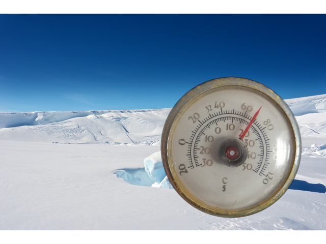
A measuring device provides us with some representation of a physical property. But how do we know that that representation is accurate ? Is the thermometer below really telling the truth ?
Calibration
For the thermometer above, can we be sure that it reads O°C when the temperature really is zero, or 100°C when that is the temperature. Even if both of these are accurate, does that bimetallic spring really change linearly over the full temperature range ? As it ages, do any of these assumptions remain true ? All of these questions are addressed by calibration. We can check the performance of the thermometer against known references. For some devices, it is possible to adjust them to correct for the differences in real and measured values, so that the display becomes accurate. For something as simple as the thermometer above, we could plot the differences in real and displayed temperature on a graph and use this to correct future readings (i.e. when the thermometer reads 32°C, we read from the graph the corresponding, corrected temperature. This approach has the advantage that it works even if the thermometer is non-linear in its response.
Zeroing, drift, and linearity are important concepts in the context of measurements and instrumentation and are compnents of calibration.
Zeroing
Definition: Zeroing, also known as nulling, refers to the process of eliminating or minimising any offset or bias in a measuring instrument. This offset is often referred to as the "zero offset" or "zero error."
Purpose: The purpose of zeroing is to ensure that the instrument gives accurate readings when the measured quantity is actually zero. It is a critical step in the calibration process and helps to correct for any inherent inaccuracies or deviations in the instrument's baseline readings.
Zeroing is a special instance of a one-point calibration. It allows us to be confident that the zero reading is accurate, but tells us nothing abut the performance of the measuring device at other values. For devices which have a very stable, linear response over their working lifetime, this may be enough. However, even these device may show drift in which case zeroing must be repeated.
Drift
Definition: Drift refers to the gradual change in the output or response of a measuring instrument over time, even when the input remains constant. This change can be caused by various factors, including temperature fluctuations, ageing of components, or changes in environmental conditions.
Compensation: To mitigate drift, instruments are often designed with compensation mechanisms or require periodic re-calibration to maintain accuracy.
Linearity
Definition: Linearity is the ability of a measuring instrument to provide output readings that are directly proportional to the input or quantity being measured. In an ideal linear instrument, a graph of input versus output would be a straight line (See Fig. 4 below).
Non-Linearity: In real-world instruments, non-linearities may occur, leading to deviations from the expected proportional relationship. Non-linearity can result from factors such as sensor limitations, electronic components, or signal processing.
By way of example, consider the clinical temperature sensors which we use. The majority of these use thermistors. As you already know the resistance of these devices changes in a non-linear fashion and generally falls with increasing temperature. Provided measurement is confined to a small range of temperaturs, this non-linearity may be very small. Fig 1 shows an exponential decay graph. Fig 2 shows a very small section of the same graph - it almost looks like a straight line. Indeed, if a line-of-best-fit is superimposed (red) it matches very well. A simple instrument might ignore the non-linearity. Provided it were used over a small temperature range, it would work well, but at the margins of its range, it would become increasingly inaccurate.
An exponential decay
A small section of the plot from Fig 1, with a line of best fit added (red)
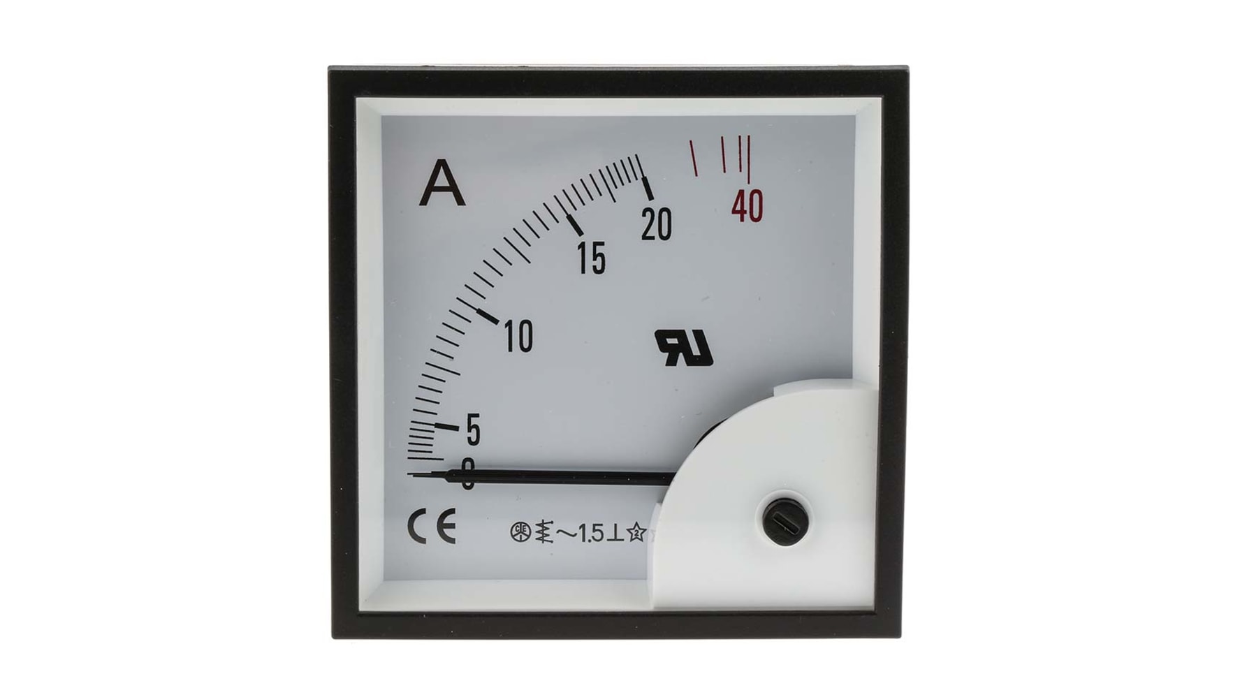
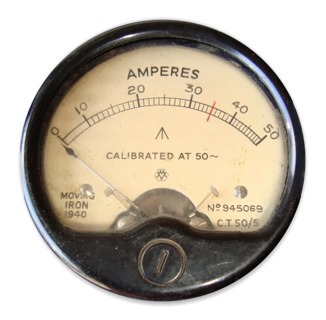
An example of an ammeter with a non-linear display. Although the instrument may have a non-linear response, its readings are still accurate
Compensation: Linearity can be improved by a number of means.
Where it arises from the instrument design (as in the thermometer example above), correction may achieved by changing other aspects of the design. Were it to use a moving coil meter to display the temperature, then the scale could be drawn in a non-linear fashion, as in the ammeter above (Fig. 3). Although the thermistor output might be non-linear and the movement of the needle also non-linear, we could still measure the temperature accurately !
In an electronic meter, the signal might be amplified in a non-linear fashion to achieve the same effect.
Where the non-linearity arises as the result of external effects or ageing of the instrument, a correction can be achieved by performing calibrations, either two-point or multi-point (Fig.4)
In summary, zeroing ensures accurate measurements at the zero point, drift addresses changes in instrument performance over time, and linearity ensures a proportional relationship between the input and output of a measuring instrument. Proper calibration, regular maintenance, and compensation mechanisms are essential to uphold the accuracy and reliability of measuring instruments in various applications. If this seems abstract, then think of what happens when you take a sample to the blood-gas machine. Often, you will find it in the process of either a one or a two-point calibration.
A calibration graph
The graph on the left represents a typical measuring device.
The red line represents the ideal - there is a perfect match between the measured values (x axis) and the 'true' value (y axis). For an ABG machine, this would mean that when the pH showed 7.35, it really was 7.35 !
Unfortunately, real machines don't always work like this. There may be a fixed offset between the real and measured information (if the relationship is linear, as shown, then based on y=mx+c this would imply an error in the value of 'c'). i.e. when the ABG machine show a pH of 7.2, the real value might be 7.3 and when the measured value shows 7.3, the real value would be 7.4 etc).
Alternatively, there may be a progressive discrepancy - i.e the value of 'm' is incorrect, so the measured and true values diverge across the full range of readings.
In the graph shown left, BOTH errors are present. There is a fixed offset between the two lines and there is a difference in the gradients. Over time, this may get worse - this is drift and requires calibrations to be repeated at regular intervals.
Click the buttons below the graph to review the implications of zeroing, one- and two-point calibrations (the text in this paragrpah will be replaced with an explanation of each action).
Damping
Most instruments take time to respond to changes in their input. We are so used to this, that we barely notice and often, it is of little importance.
Set:
Sample:
The meter behaves as a realistic moving-coil meter, but you can choose the level of damping. Press each of the 'Sample' buttons and see what happens; the reading will reset after a few seconds.
Both under-damping and overdamping delay our ability to get a reliable reading from this meter, whereas when it is 'critically damped', the needle moves to the correct value as quickly as possible with no overshoot. Hover, the effects of over or under-damping can be much more important. If you imagine that we are using this meter to record an invasive blood pressure (rather improbable, but bear with it). Clicking on the 'Under-damped' button results in the needle overshooting the real value and then swinging back and forth around it. You will have seen this behaviour on an arterial line trace. When the system is under-damped, the trace appears 'spiky' and you may notice additional waves which correspond with the resonance you can see in the meter's needle. This is important, because our monitors are programmed to measure the peak pressure as the systolic and they will misinterpret the maximum value as being real. It isn't. It is the overshoot from an under-damped system just as you can demonstrate from this meter. The MAP will also be affected. As a result, it is possible to run a patient hypotensive despite having a perfectly acceptable invasive BP on the monitor.
An under-damped system also creates artefacts. In the meter, you see that the needle reaches the correct reading eventually, but what if we are reading a parameter which is changing quickly such as blood pressures ? In this case the meter may never catch up with the true reading and it will always under-read. The arterial waveform will appear 'rounded'. Again this is something that you will encounter often with arterial lines and can be difficult to detect as the onset can be insidious as the cannula becomes partially occluded.
Hysteresis
If you imagine that the meter above has rather poor bearings, then as the mechanism approaches the correct reading, there may be too little energy available to overcome the friction and the needle will stop short.
Whether the needle stops above or below the true reading will depend on whether it was swinging to the right or left (if swing to the right, then it will under-read, if to the left, then it will over-read - i.e. it always stop short of the true value). This difference between readings depending upon whether the needle is rising or falling is hysteresis. Although I have described it in terms of a moving coil meter, it applies to many systems, both analog and digital. I have chosen the example of a meter because it is easy to imagine.
Heater controller.
Specify temp:
Heater status: Unplugged !
Use hysteresis
Click the slider to activate, anywhere else in the page to deactivate
Hysteresis is widespread - and on occasion is there by design. Without hysteresis, a fluid warmer (below - click on the slider to start it) would be behave in very strange ways. As it reached its switching threshold (either on or off - in the example, set at 43°C)) it would become unstable, rapidly switching between on and off as the random noise in the system (see below) caused it first to exceed the switching threshold, then revert. If we build in positive feedback (hysteresis), then it might only switch on when the fluid temperature fell below 42°C and switch off when it exceed 44°C.
Biological potentials
Many tissues are electrically active and it is useful to be able to monitor some of these (heart, brain, muslce etc.). Unfortunately, the magnitudes of these signals is small, both in terms of voltage and current and both of these are important when try to record data.
Source
Typical magnitude
ECG
0.5-2.0mV
EEG
δ (0.5-4Hz)
20-200µV
θ (4-8Hz)
20-100µV
α (8-13Hz)
20-60µV
β (13-30Hz)
5-20µV
γ (30-100Hz)
1-10µV
EMG
Surface
50µV-50mV
Intramuscular
100µV - 10mV
Magnitudes of biological signals
Voltage
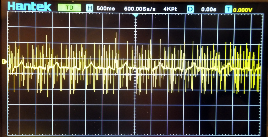
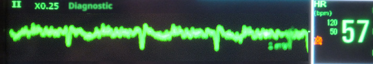
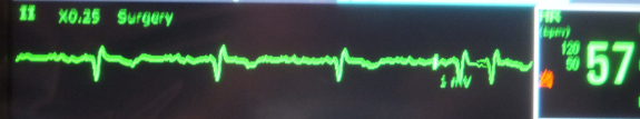
Typically, the signals will have to be amplified by 2-4 orders of magnitude. Unfortunately, some random interference 'noise' will always be present, either from external sources such as mains interference, diathermy or even random fluctuations from within. As the wanted signal is amplified, so is the unwanted. By way of example. see Fig 5a. This is an ECG signal seen on an oscilloscope. It has been amplified to make it visible and there is an awful lot of interference ! Exactly the same signal is then shown displayed on a medical monitor, both in 'diagnostic' and 'surgery' mode (although sadly, the former is rather a poor quality picture). On the monitor, the level of noise is greatly reduced by the application of filters. However, this also results in the loss of some information and details such as pacing spikes may be lost. As a result, many moinitors will off different levels of filtration such as 'Diagnositic' (low filtration - most of the detail is preserved, but so may be interference), 'surgery' (high level of filtration which will minimise diathermy interference, but will also damp other, high-frequency information).
Managing noise in amplified signals
Just as interference is amplified, so is any voltage 'offset'. Fig. 6 shows a small ECG trace (blue) centred around the baseline (0V). When amplified, this gives the signal shown in red (click the 'Amplify' button). Often, however, DC offsets can be present and can be generated by items such as the ECG electrodes (click the 'Add offset button').
When this offset ECG is amplified (click the 'Amplify' button again), the offset is also amplified and the trace disappears off the monitor screen !
Effect of amplification when a DC offset is present
In order to improve the signals, we use filters and these consist of components with which you are already familiar.
Inductors can remove high frequency signals (high-pass filter) and so this is what is used to remove diathermy interference.
Capacitors can block low-frequency and DC signals (low-pass filter). If the offset is large, it takes time for the capacitor plates to charge and so there is a delay before the signal reappears on your monitor. Click the 'Reset' buttons and then select the 'Use capacitor' checkox in Fig 3. If you amplify the signal again, nothing seems to be different - nor should it; there is no DC offset to block and so the capacitor does nothing. Now click the 'Add offset' button again and you will notice that the ECG signal starts with an offset, but quickly returns to the baseline as the capacitor charges and then blocks the DC component. Now try to amplify the signal and it should remind you of a pattern you will have seen on your monitor. The ECG waveform gradually settles back to the baseline, following an exponential decay pattern. This happens because the coupling capacitor is charging. As it approaches the (constant) offset voltage, the charge current falls to zero. The AC signals can stall pass unchanged. But why does it take so long ? Well this happens because of the next issue - current. Since we cannot draw any significant current from a biological syste, the monitor must have a very high input resistance. As a result, very little current can flow and even with a small capacitor, charging will take time.
Combining a high-pass capacitor filter with a low-pass indictive filter provides a 'band-pass' filter, which aims to pass the frequencies in which we are interested and block all others.
Current
The best way to think about the effects of current is to consider cells as little batteries. EVERY battery has some internal resistance and we should draw batteries as shown in Fig 7.
Under normal conditions, batteries are chosen so that in use, their expected current is never so high that a significant proportion of their voltage appears across this 'internal' resistance. This is the situation in Fig 8, where the circuit current is relatively low and the voltage across the load is close to the battery rating.
If the battery is excessively loaded, then the picture is closer to that in Fig 9. Here the circuit current is limited by total resistance Rint+Rload, BUT since Rload is much smaller than Rint, most of the battery voltage appears across Rint which we can't measure. If we measure measure the voltage across the load, it will be much lower than the battery's rating. Given time, then the energy dissipated in the battery may result in overheating, fire or explosion.
A realistic representation of a battery
A battery under light load
A battery under excessive load
An old moving-coil meter - perhaps a little to large for biological use !!
A battery under excessive load
What has this got to do with cells and our ability to measure biological signals ? The answer is that most meters draw some current from the circuit under test. Fig 10 shows a very old, moving coil meter. The energy to move the needle is drawn from the circuit under test. Using this meter would create the same situation as in Fig 9 and any reading would be meaningless. To measure biological signals, we require meters which draw very little or even no current. This can be another use of the Wheatstone bridge; when the two arms of the bridge are balances (i.e. no current through the meter, then the voltages in the two are balanced. The Wheatstone can be disconnected and voltages measured in the Wheatstone will be the same as those in tissue under investigation.